Version 0.9 · Preprint / Framework Paper · FORSCH-PROV0420 (number provisional) · as of 6 Oct 2026
| Field | Entry |
|---|---|
| Author | Thomas Schüller (researcher), ORCID 0009-0003-9799-6747 |
| Author imprint | Thomas Schüller · Syntagma Forschung · Vienna (no separate legal entity) |
| Affiliation | Independent researcher, no institutional affiliation |
| Correspondence | forschung@tschueller.com |
| Repository | forschung.tschueller.com · syntagma-science.com |
| Funding | self-funded |
| Conflicts of interest | none |
| Licence | CC BY 4.0 |
| Data status | no experimental raw data; ten numerical minimal models, reproducible (Section 14, Appendix C) |
| Source status | 50 entries verified (publisher, standards register, full text), 12 flagged as open in Appendix I.2; these concern almost exclusively the edition and ISBN of textbooks and first editions |
| Track | FORSCHUNG (open channel, feeder). Tools run exclusively on the syntagma-science platform, see Appendix G |
This version claims no new fundamental physics. It is an ordering framework for the measurability, reconstructability and falsifiability of physical measurement chains.
Nothing in the work itself. No result, no proof, no figure and no appendix has changed. This version makes the bundle around the work ready for publication; the number is carried along so that work and bundle do not drift apart.
| No. | Change | Reason |
|---|---|---|
| 1 | New VEROEFFENTLICHUNG.md in the main
folder: the sequence in one place — the seven decisions that block
everything, the order platform → deposit → journals, tick-off steps per
track |
the sequence was spread across the handover, the operations manual and the upload notes; when publishing you need it in one place |
| 2 | Landing page extended with legal matters: imprint, terms of use, privacy, separate licences for work and tool, liability note | without these a page is not publishable |
| 3 | Landing page extended with the network of brands | whoever cites, cites Syntagma; whoever licenses, buys from the responsible track. That was stated nowhere |
| 4 | Citation template in the author register corrected — it still read Version 0.3 — and extended with per-version check points | an outdated citation template produces wrong citations, permanently |
The material is finished. What remains are the seven
decisions in VEROEFFENTLICHUNG.md Section 1; all of them
belong to the author and none can be derived from the material.
This version changes no result and no proof. It draws the disclosure line explicitly instead of presupposing it.
| No. | Change | Reason |
|---|---|---|
| 1 | New Appendix G.6: self-protection and the disclosure line per REGEL-PROV0002 | the work sits beside a paid offering; leaving that unstated leaves open whether something is being held back |
| 2 | For every component it is stated whether it is open and why — including what is not present at all | a claim without evidence would be advertising; evidence without a line would be a build manual |
| 3 | Checkability outranks protection is recorded as the precedence | a framework that cannot be refuted supports no offering |
| 4 | The choice for the browser tool is made and justified: MESSWERK stays open on the platform page | “in the browser” and “computing core internal” exclude each other; the rule requires a deliberate choice rather than a tacit one |
| 5 | REGEL-PROV0002 sits as its own file in the bundle; the adoption block now covers both rules | it governs all tracks, not only this project |
Substantively unchanged: measurement chain, Theorems 1 and 2, classification A/B/C, numerics, experimental protocol, references, source checklist, licence levels, active/passive assignment.
This version changes no result and no proof. It anchors a cross-track rule that so far existed only as a decision.
| No. | Change | Reason |
|---|---|---|
| 1 | New Appendix G.5: active and passive versions per REGEL-PROV0001 | the line for what may go on a deposit was described for this project but not stated as a general rule |
| 2 | The borderline case of computation scripts is settled: they are passive and stay on the deposit | without them the work could not be checked, and checkability is the reason for depositing at all |
| 3 | The difference between free verification and the licensed tool is stated in G.5 rather than assumed | anyone verifying the numbers here does not need the tool; the tool computes on someone else’s measurement chain |
| 4 | The rule sits as its own file in the bundle
(regelwerk/), with an adoption block for the central
rulebook |
it governs all projects, not only this one |
Substantively unchanged: measurement chain, Theorems 1 and 2, classification A/B/C, numerics, experimental protocol, references, source checklist, licence levels.
This version changes no result and no proof. It converts the commercial arrangement to a platform-centred one.
| No. | Change | Reason |
|---|---|---|
| 1 | Appendix G rewritten: syntagma-science is the destination, the open research channel the feeder | tools now run exclusively on the platform; Zenodo carries no tool, not even a preview build |
| 2 | Licence levels L0–L3 and six product classes per LIZ-PROV0001 added as Appendix G.2 and G.3 | the assignment existed only as four service levels in the offering, not in the work itself |
| 3 | Appendix H reordered: platform → deposit → journals | a reference needs a destination; the platform has to exist before the deposit |
| 4 | Zenodo bundle prepared separately (Appendix H.2,
folder zenodo-upload/) |
the working bundle and the publication bundle are not the same; only the open material belongs on the deposit |
| 5 | Every deposit of the preprint carries the reference to syntagma-science | the preprint is a reach channel, not an end in itself |
Substantively unchanged: measurement chain, Theorems 1 and 2, classification A/B/C, numerics, experimental protocol, references, source checklist.
This version changes no result and no proof. It folds in the source check that version 0.4 listed as the single remaining open task.
| No. | Change | Reason |
|---|---|---|
| 1 | ISO 12233:2023 → ISO 12233:2024 in Section 19.3, Section 19.6 and Appendix D | the fifth edition supersedes the 2023 edition and also carries a changed title: “Digital cameras — Resolution and spatial frequency responses” |
| 2 | IEC TR 60825-14:2022 (Ed. 2.0) in place of the undated reference; status of IEC 60825-1 Ed. 4 noted | an undated normative reference is not reproducible in an experimental protocol |
| 3 | Mezghani, Antreich & Nossek (2010): the conference paper WSA 2010, Bremen, 143–150, DOI 10.1109/WSA.2010.5456454 is now the primary source, arXiv:1010.5532 the preprint | the factor in class B now rests on the reviewed version |
| 4 | Kalman (1963): journal name corrected to Journal of the Society for Industrial and Applied Mathematics, Series A: Control | SIAM Journal on Control is the later name of the same journal, not yet in use in 1963 |
| 5 | Six missing DOIs added: Krener & Ide, Galiffi et al., Hansen, Janesick, Stadler, Amari (2016) | these had no identifier in v0.4, or only an unverified ISBN |
| 6 | Issue numbers added for ten entries (among them Paris, Bellman & Åström, Berreman, Shannon, Landauer, Hempel) | the page range alone does not identify the volume unambiguously |
| 7 | Appendix D converted into one continuous alphabetical list | the split into “DOI-verified” and “further sources” lost its purpose once the check was done |
| 8 | Appendix I restructured into I.1 verified, I.2 still open, I.3 what the check changed in the work | the reader should see the remaining gaps at a glance |
| 9 | Open entries reduced from 25 to 12, verified entries from 23 to 50; those remaining concern almost exclusively the edition and ISBN of textbooks and first editions | the sources that carry content are now fully substantiated |
What is still outstanding: the choice of edition for fourteen textbooks and three first editions, the edition status of JCGM 100/200 and EMVA 1288, and the access date of the SEP entry. These are itemised in Appendix I.2 and are to be closed before a journal version.
| No. | Change | Reason |
|---|---|---|
| 1 | The gap claim is everywhere tied to the literature strands searched rather than stated absolutely | Integrity: the search was not exhaustive |
| 2 | Class C extended by three cases: EMCCD at low gain, quantisation outside the limiting cases, generally heteroscedastic noise | completeness of the classification |
| 3 | Section 5.5 extended by the noise coefficient (Chao, Ward & Ober) and the Stam inequality | two further neighbouring concepts requiring demarcation |
| 4 | New Section 7.1: Rayleigh and Sparrow as special cases of a threshold on | the Fisher information is the sharper criterion; the classical criteria can be placed rather than discarded |
| 5 | Convention for the excess noise factor stated explicitly | Robbins & Hadwen define , other works the squared quantity — without a convention the factors 2 and 1/2 are not traceable |
| 6 | Quantum bounds under noise (Escher et al.) and monotonicity of the quantum Fisher information under CPTP maps added | connects Section 13 to the data-processing inequality |
| 7 | New Appendix H: publication path, with a venue matrix and the arXiv endorsement rule changed on 21 January 2026 | so far only noted in the handover |
| 8 | New Appendix I: source checklist with a status per entry | separates verified from unverified references traceably |
| 9 | References extended by twelve entries | Chernoff, Amari (2001), Chao et al., Hynecek & Nishiwaki, Mortensen et al., Escher et al., Paris, Gan & Law, Aspden et al., Worrall, Earman & Norton, Stadler |
| No. | Change | Reason |
|---|---|---|
| 1 | The core statement is explicitly identified as observational equivalence in the sense of Rothenberg (1971) and no longer framed as an own finding | Literature check: the statement has been standard since 1971. The contribution lies in the transfer to physical measurement chains, not in the statement |
| 2 | The separability criterion is formulated as Theorem 1 with an equivalence proof instead of being asserted | On a connected product domain, is equivalent to the product form |
| 3 | Sharper formulation via stage efficiencies (Theorem 2) | The telescoping identity is trivial. The real claim is that depends only on its own stage’s parameters |
| 4 | Classification of forward models into three classes with evidence and counterexamples (Section 5.6) | The open question from v0.2 is thereby settled for the main channel classes |
| 5 | Demarcation from parameter orthogonality (Cox & Reid 1987) and from cascaded-detector theory (DQE) | These are the closest literature strands; the DQE literature explicitly denies the general product form |
| 6 | Four new numerical minimal models M7–M10 with Figures 6–9 | Stage efficiency, separability map, qubit dephasing, slit experiment |
| 7 | Complete experimental protocol for the optical slit experiment (Section 19) | v0.2 named the experiment only as an open item |
| 8 | New section Vienna lineage and the philosophy of measurability (Section 16) | Mach, Boltzmann, Bridgman, Vienna Circle, Schrödinger, modern measurement theory |
| 9 | New section demarcation from observability theory (Section 17) | Kalman and Hermann–Krener are the closest competing formulation |
| 10 | References extended with DOIs; Appendix F states what was not found in the literature | Positioning of the contribution |
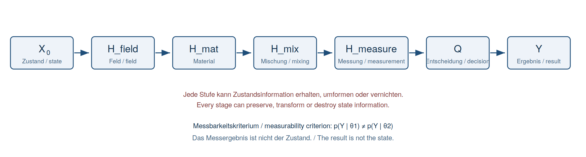
This work formulates an information-based ordering framework for physical measurability and reconstructability. The claim is not to introduce new fundamental physics but to organise established concepts from wave theory, electrodynamics, scattering theory, signal theory, digitisation and quantum measurement along a common measurement chain:
The starting point is observational equivalence: if for , unique reconstruction from that channel is excluded. This is not new; it is the definition of identifiability of a parametric model, and its local version has been equivalent to regularity of the Fisher information matrix since Rothenberg (1971). The contribution of this work lies in two points.
First, the diagnostic working quantity is defined as an effective signal-to-noise ratio and derived exactly from the Fisher information for the scalar Gaussian channel: with one obtains . Second, the product form
receives a testable validity criterion: on a connected product domain it is exact precisely when is additively separable. Stated more sharply via stage efficiencies , the claim is that each depends only on the parameters of its own stage. This is decided for three classes of forward models: multiplicative transmission with single-stage noise and Poisson thinning satisfy the criterion exactly; high-gain EMCCDs and low-SNR one-bit quantisation satisfy it asymptotically; multi-stage noise injection, the crossover between shot and read noise, nonlinearity and saturation violate it.
Ten numerical minimal models with a fixed random seed support the statements, among them a separability map over signal level and read noise and a fully computed optical slit experiment. The scientific load-bearing capacity lies in the falsification conditions.
Keywords: measurability; reconstructability; identifiability; observational equivalence; Fisher information; separability; cascaded systems; wave-vector transfer; coherence; inverse problems; quantum measurement.
Physical measurements are often described through single terms: signal strength, frequency, wavelength, reflection, resolution, noise, detection. These are necessary but not sufficient. A strong signal may say little about the state sought. A local null signal may arise from destructive interference. A digitally crisp result may rest on coarse quantisation or algorithmic priors. A reflected signal may carry energy while having lost direction and phase.
The central question is therefore not whether a signal exists, but:
Which state information is distinguishable in the signal under the given physical and instrumental conditions?
The contribution is not a new law of nature. It is a framework that orders existing physical descriptions along the question of measurability and — since version 0.2 — states the conditions under which the working quantity used is admissible. Version 0.3 answers that question for the main channel classes.
The model claims no new fundamental physics. It replaces neither Maxwell’s equations, nor quantum mechanics, scattering theory, Fourier optics, information theory, nor the theory of inverse problems. It is an ordering framework whose purpose is to make the measurement question explicit:
| Symbol | Meaning |
|---|---|
| physical initial state | |
| field or wave propagation | |
| material response: reflection, transmission, absorption, scattering, dispersion | |
| mixing, multiple scattering, mode coupling, nonlinearity, linear time variance | |
| measurement process, detector response, measurement operator | |
| quantisation, thresholding, classification, digital decision | |
| registered result |
In the linear case with (2). If has a null space, different states produce the same signal. In the nonlinear case (3), and local sensitivity decides.
A signal carries state information about if
and unique reconstruction is excluded if
Provenance of the statement. Equation (5) is the definition of observational equivalence of two parameter values; a model is identifiable if no two distinct parameter values are observationally equivalent. Rothenberg (1971) shows that under weak regularity conditions local identifiability is equivalent to non-singularity of the Fisher information matrix. This work adopts that theorem and applies it to physical forward chains. The contribution lies in the transfer and in the stage decomposition, not in the statement itself.
Three levels must be separated:
| Level | Criterion | Quantity |
|---|---|---|
| measurability in principle | identifiability | |
| practical reconstructability | overlap of distributions | Kullback–Leibler divergence, |
| robust technical estimability | achievable variance | Fisher information, Cramér–Rao |
In the quantum case the Fisher information is replaced by the quantum Fisher information; Braunstein and Caves (1994) show that the statistical distinguishability of neighbouring states defines a Riemannian metric on the space of density operators.
is defined as the effective signal-to-noise ratio of the equivalent Gaussian channel that yields the same Fisher information about as the measurement chain under consideration.
Hence
is, in the anchor case, not an approximation but exactly the Shannon capacity of the equivalent channel.
For , , (7). With the dimensionless definition and
it follows exactly that
is therefore the Fisher information with respect to , and is the logarithmic sensitivity (elasticity) of the forward chain. If the further stages act as amplitude-scaling factors without changing noise power, then and
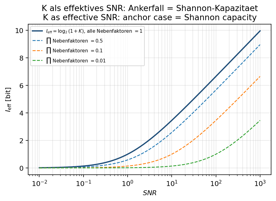
| Factor | Meaning | Range |
|---|---|---|
| signal-to-noise ratio of the carrier | ||
| resolution or structure-transfer factor | ||
| material and propagation factor | ||
| coherence factor, | ||
| bearing-information factor | ||
| normalised state–signal coupling | real |
Let be positive and twice continuously differentiable on a connected product domain . Then the following are equivalent:
Proof (sketch). (1) (2): ; each summand depends on exactly one variable, so all mixed second derivatives vanish. (2) (1): if all mixed second derivatives of a function vanish on a connected product domain, then is a function of alone; integration yields .
The criterion is therefore not sufficient or necessary but equivalent to the product form. It is invariant under coordinatewise reparametrisations , but not under mixing transformations. Whether, for a given model, a mixing reparametrisation exists that makes separable is a boundary-value problem of the same kind as the orthogonalisation of Cox and Reid (1987); it remains open.
For a chain with Fisher informations about , the telescoping identity always holds:
The bound follows from the data-processing inequality for Fisher information (Zamir 1998). Identity (11) is therefore trivial and by itself carries no content. The substantive claim of the framework is:
The stage efficiency depends only on the parameters of its own stage — not on upstream parameters and not on the signal level.
Only in this form is the product form a testable physical statement about channel structure. It is equivalent to Theorem 1 applied to the parameter groups of the individual stages.
| Concept | Object | Relation to the criterion |
|---|---|---|
| Parameter orthogonality (Cox & Reid 1987) | off-diagonal of the Fisher matrix between interest and nuisance parameter | Logically independent: may factorise in while , and vice versa. Only the reparametrisation question is shared |
| Data-processing inequality (Zamir 1998) | does not increase along a Markov chain | Gives , but no product rule |
| Stam inequality, chain rule | and additive decompositions | Additive, not multiplicative: information adds inversely, not as a product |
| Noise coefficient (Chao, Ward & Ober 2012) | ratio of the pixelwise Fisher information to the ideal Poisson case | Closest to the criterion: an efficiency per stage. But defined signal-dependently and silent about the cascade — exactly the gap Theorem 2 closes |
| Noise-figure cascade (Friis 1944) | Additive with gain weighting — the standard case of a violation | |
| Cascaded detectors, DQE (Rabbani, Shaw & Van Metter 1987; Cunningham & Shaw 1999) | signal and noise power spectra per stage | Closest chain decomposition. It works with second moments rather than Fisher information and states that the DQE of a cascaded system is generally not a multiplicative cascade of individual DQEs |
| Class | Forward model | Criterion (10) | Evidence |
|---|---|---|---|
| A — exact | multiplicative transmission , noise from exactly one stage, parameter-independent | satisfied | |
| A — exact | Poisson with thinning, | satisfied | binomial thinning preserves the Poisson form; |
| B — asymptotic | EMCCD at high gain | satisfied with constant factor | excess noise factor (Robbins & Hadwen 2003) |
| B — asymptotic | one-bit quantisation at low SNR | satisfied with factor | Mezghani, Antreich & Nossek (2010), WSA, DOI 10.1109/WSA.2010.5456454 |
| C — violated | noise injected at several stages, | violated | Friis structure; cross terms between and |
| C — violated | crossover between shot and read noise, | violated in the crossover | numerically in Section 14.7 |
| C — violated | aperture limitation: and both depend on | violated | double counting of the same physical resource |
| C — violated | nonlinear characteristic, saturation | violated; at saturation | with |
| C — violated | gain-dependent noise | violated | numerically in Section 14.4 |
| C — violated | EMCCD at low gain | violated | the excess noise factor depends on and the effective read noise is ; acts on signal and noise term at once |
| C — violated | quantisation outside the limiting cases, medium to high SNR | violated | the loss factor then depends on SNR, no longer on the quantiser alone |
| C — violated | generally heteroscedastic noise | violated | additional term per Equation (12) |
This three-class assignment rests on the literature strands searched — data-processing inequality, cascaded systems, quantisation, detector noise — and claims no completeness over all conceivable channel classes.
The general reason for class C fits in one line: for ,
The second term is absent from . As soon as one parameter acts on both signal and noise, it contributes to both terms and the factors are no longer independently calibratable.
Convention for the excess noise factor. Robbins and Hadwen (2003) define the excess noise factor as an amplitude quantity with at high gain; other works, such as Mortensen et al. (2010), already quote the squared quantity. This work consistently carries the squared quantity as a variance factor: the variance grows by , the Fisher information falls by . For a high-gain EMCCD this gives and the factor in class B.
Direction is determined relative to an axis, aperture, source, detector or interface. For a wave with wave vector and observation axis :
For two counter-propagating components along the signed direction balance is
is not a new quantity but the net flux normalised to total power. With reflection coefficient and standing-wave ratio , exactly
is thus a rescaled VSWR reading, directly measurable in any RF laboratory (checked numerically in 14.5).
Near-field methods, structured illumination, nonlinearity, repeated measurements or priors extend this bound. They are not violations of the model but additional information channels that must be entered into the chain explicitly.
The classical resolution criteria of Rayleigh, Sparrow and Abbe are formulated for incoherent point sources and impose a fixed threshold: resolved or not. The Fisher information knows no such threshold; it falls continuously. Both descriptions can be reconciled rather than played off against each other.
For two point sources at separation , locally , and is the normalised separability of detection theory. A classical criterion is then the statement that reaches a particular value:
| Criterion | classical form | form within the framework |
|---|---|---|
| Rayleigh | the first minimum of one diffraction pattern falls on the maximum of the other | exceeds a threshold depending on photon count and noise model |
| Sparrow | the dip between the maxima vanishes | a stricter threshold on the same quantity |
| Abbe | falls below a value at which drops under one bit |
The gain of this reformulation is practical: the classical criteria know nothing of photon count. They say the same for an image with ten photons and one with ten million. The Fisher form says how many photons are needed for two states to become distinguishable at a given aperture — and that is the question actually asked in design.
is an energy balance, not an information balance. A mirror preserves directed information; a matte surface may return a similar amount of light while diffusing direction and phase. describes how much of the signal structure usable for the state question arrives ordered at the detector.
Destructive interference means that field contributions add vectorially to zero at the point considered. A local null signal is not a global proof of absence.
| Medium class | New field frequencies? | Mechanism |
|---|---|---|
| linear, time-invariant (LTI) | no | pure superposition |
| linear, time-varying (LTV) | yes | parametric coupling to the modulation |
| nonlinear | yes | mixing products, intermodulation |
Morgenthaler (1958) solves Maxwell’s equations for media with time-dependent permittivity and permeability and shows that the fields remain linear when the medium parameters do not respond to field strength, yet a monochromatic wave undergoes a frequency deviation. Parametric amplifiers, modulators, switched plasmas and time-modulated metamaterials (Galiffi et al. 2022) belong to this class. With , by contrast, mixing products and intermodulation arise.
In the linear, isotropic, local limit , , . In anisotropic, dispersive, nonlinear or time-dependent media, , , must be modelled as tensors, frequency functions, convolution kernels or nonlinear response functions. In this section denotes permeability only; the coherence factor is .
If is pure post-processing of the same analogue signal, the data-processing inequality holds:
Digitisation creates no physical state information that is contained neither in the analogue signal nor in additional data, priors or further measurements.
The corresponding estimation bound is the quantum Cramér–Rao bound (Helstrom 1969); the distinguishability metric is formulated by Braunstein and Caves (1994), with . An accessible overview for applications is given by Paris (2009).
The quantum Fisher information is monotone under completely positive, trace-preserving maps; this is the quantum form of the data-processing inequality of Section 12 and the reason also holds in the quantum case. For estimation bounds under noise there is a general framework (Escher, de Matos Filho & Davidovich 2011); under dephasing the attainable scaling falls back asymptotically to and the Heisenberg advantage is lost. Decoherence means that phase relations become practically inaccessible through coupling to detector or environment; one then considers . All purifications of a reduced state are related by unitaries on the ancilla (Hughston, Jozsa & Wootters 1993): infinitely many total states yield the same local statistics. That is the quantum case of Equation (5).
Figures from
werkzeuge/FORSCH-PROV0420_minimalmodelle_v0.2_2026-08-26_numerik.py
(seed 20260826, models M1–M6) and
…_v0.3_2026-10-05_numerik.py (seed 20261005, models
M7–M10). Raw results: ergebnisse.json and
ergebnisse_v0.3.json.
Model , , , , .
| Quantity | Value | Check |
|---|---|---|
| analytic | 4.000 | — |
| Monte Carlo (score variance) | 3.991 | deviation 0.23 % |
| Cramér–Rao | 0.2500 | — |
| empirical variance of the ML estimator | 0.2494 | deviation 0.23 % |
| 4.000 | identical to | |
| 2.322 bit | Shannon anchor | |
| at coupling | 0 | Equation (5) |
, : Fisher eigenvalues , null-space direction . Replacing the exact null space by a small singular value , the Cramér–Rao bound grows as (from 0.1 at to at ).
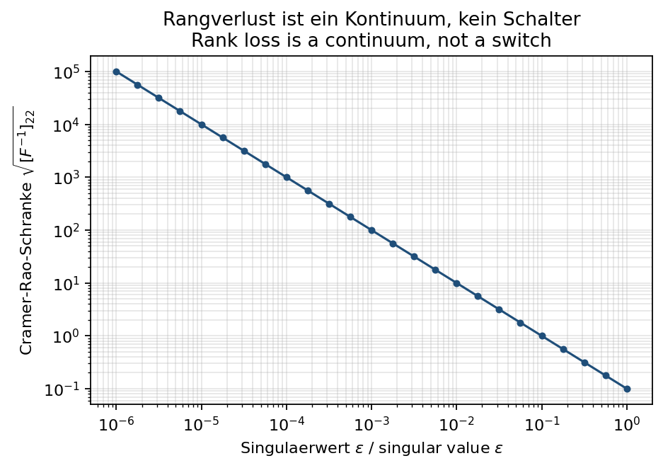
What decides is the singular-value spectrum relative to the noise level — the Picard condition of inverse-problem theory (Bertero & Boccacci 1998).
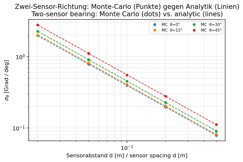
, m/s, µs, per point.
| [m] | [°] | Monte Carlo [°] | analytic [°] | |
|---|---|---|---|---|
| 0.00 | any | — | — | 0 |
| 0.05 | 0 | 0.787 | 0.786 | |
| 0.05 | 30 | 0.906 | 0.908 | |
| 0.05 | 60 | 1.590 | 1.572 | |
| 0.20 | 0 | 0.197 | 0.197 | |
| 0.20 | 30 | 0.227 | 0.227 | |
| 0.20 | 60 | 0.395 | 0.393 |
Median relative deviation 0.20 %, maximum 3.4 %.
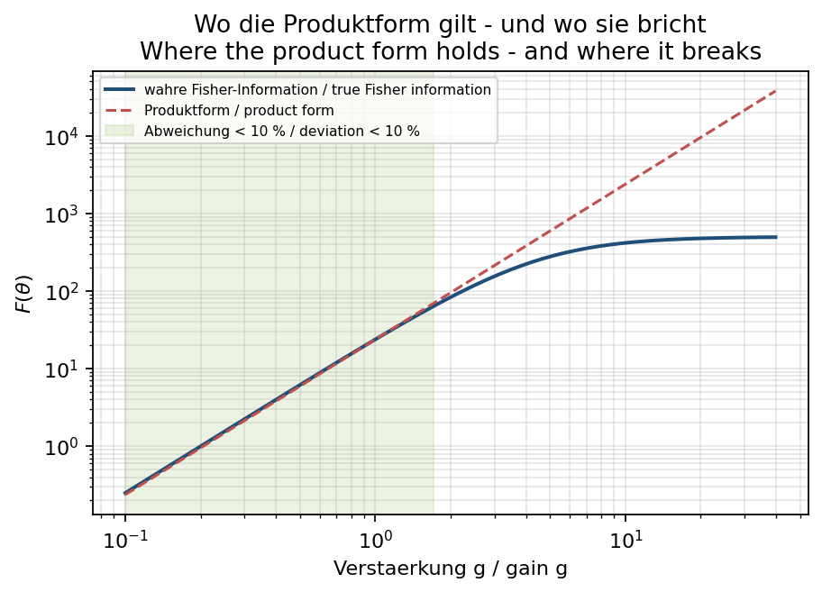
, , . The true Fisher information saturates at 500; the product form calibrated at grows as .
| Gain | Behaviour | Relative deviation |
|---|---|---|
| 0.1 … 1.71 | product form usable | < 10 % |
| 10 | product form overestimates | 436 % |
Identity (15) checked over ; maximum deviation (machine precision).
| VSWR | ||
|---|---|---|
| 0.0 | 1.0 | 1.000 |
| 0.2 | 1.5 | 0.923 |
| 0.5 | 3.0 | 0.600 |
Poisson source photoelectrons, three transmission stages with nominal , read noise at the end of the chain. Measured: .
| [] | maximum deviation from nominal transmission | |||
|---|---|---|---|---|
| 0 | 0.800 | 0.600 | 0.500 | 0.0005 |
| 5 | 0.795 | 0.588 | 0.477 | 0.023 |
| 50 | 0.679 | 0.399 | 0.272 | 0.228 |
| 200 | 0.643 | 0.363 | 0.252 | 0.249 |
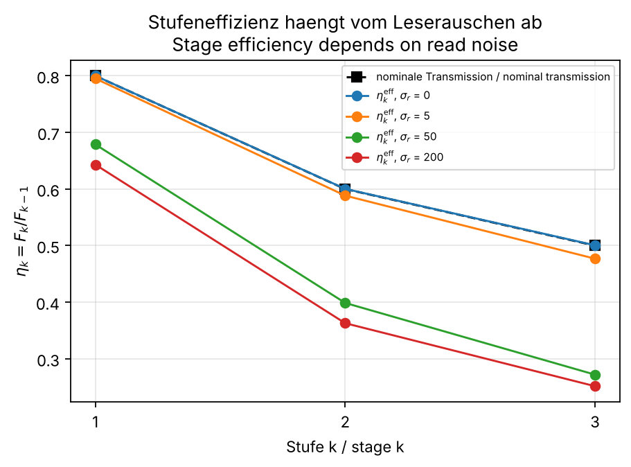
This is Theorem 2 in numbers. Without read noise, is exactly the nominal transmission of its own stage and the product form holds. With read noise, depends on how much signal stages 1 and 2 left behind — the stage efficiency is then no longer a stage property, and the factors cannot be calibrated separately.
Mixed second derivative over signal level and read noise, grid 120 × 120 over and .
| [] | [] | Regime | |
|---|---|---|---|
| 10 | 1.0 | 0.173 | crossover |
| 10 | 102 | 0.002 | read-noise limited |
| 962 | 1.0 | 0.002 | shot-noise limited |
| 962 | 9.7 | 0.163 | crossover |
| 100,000 | 9.7 | 0.002 | shot-noise limited |
| 100,000 | 102 | 0.178 | crossover |
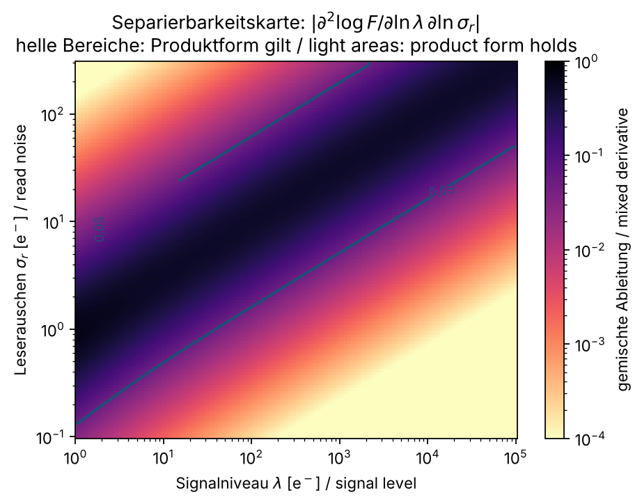
At a threshold of 0.05, 58 % of the parameter area considered is separable. The structure is instructive: separability holds in the two asymptotic regimes — clearly shot-limited or clearly read-limited — and breaks in the crossover band . The product form is therefore not an either/or but a property of the operating point. In practice: factorisation is admissible where one noise contribution clearly dominates.
State with , .
| Quantity | Value |
|---|---|
| for | |
| optimal single duration at fixed total time, theoretical | |
| same quantity, numerical | 0.500 |
| at | 0.3679 |
| of a projective measurement at | 0.3679 (attains to grid resolution ) |
| at | 0 |
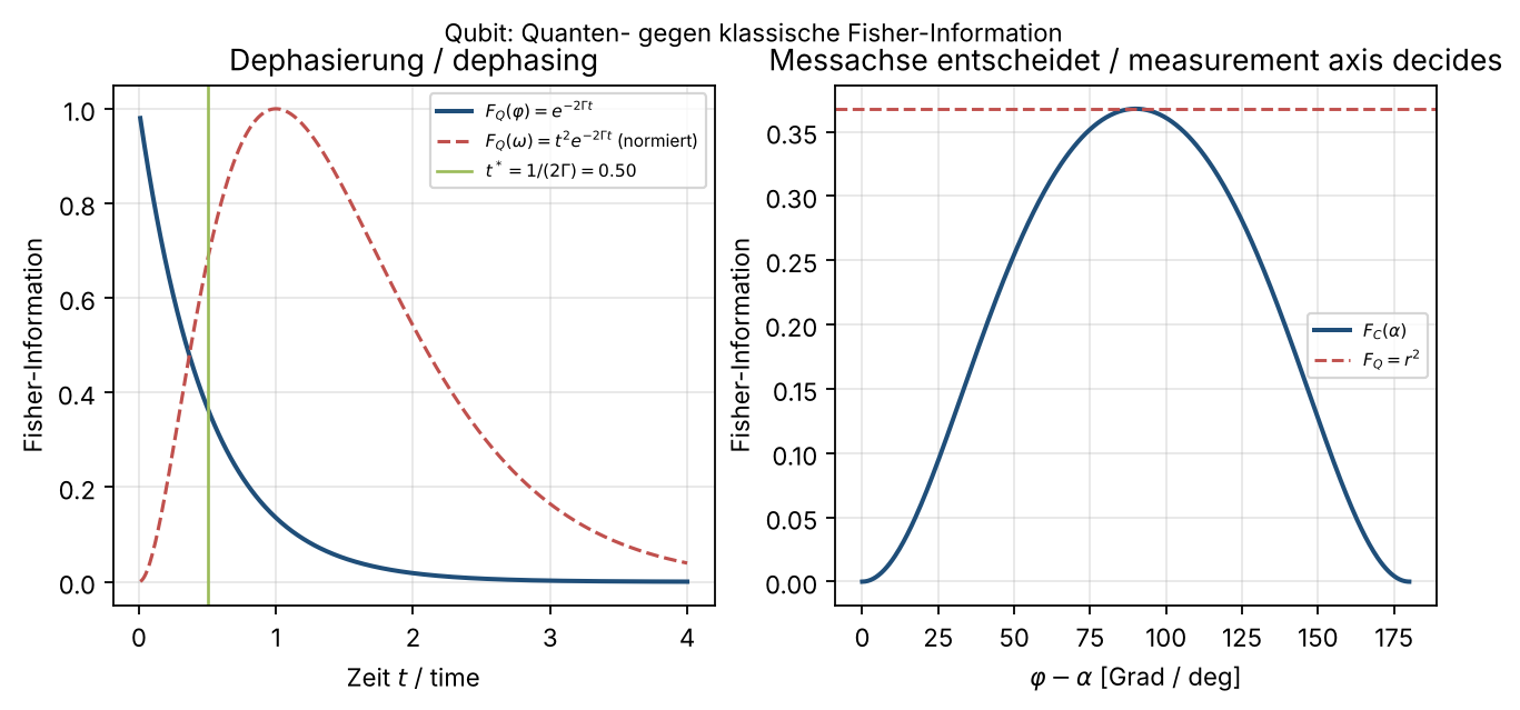
Two lessons for the framework. First, non-distinguishability in the quantum case is measurement-relative: at , although — the information is present in the state and inaccessible in the chosen channel. Second, with shows that the separability criterion is violated in the parameters but satisfied in . Admissibility of the product form depends on the choice of parametrisation.
Single slit, µm, nm, m, pixel 1.55 µm, 4096 pixels, read noise 3 , conversion 1 /ADU, peak signal 4000 , pixel integration with 16 nodes.
| Quantity | Value |
|---|---|
| Fraunhofer number | 0.035 (condition satisfied) |
| position of | 0.690 mm |
| first minimum | 4.333 mm |
| Fisher information | |
| Cramér–Rao bound | 35.7 nm |
| Monte-Carlo standard deviation of the ML estimator () | 35.2 nm |
| Cramér–Rao efficiency | 1.03 |
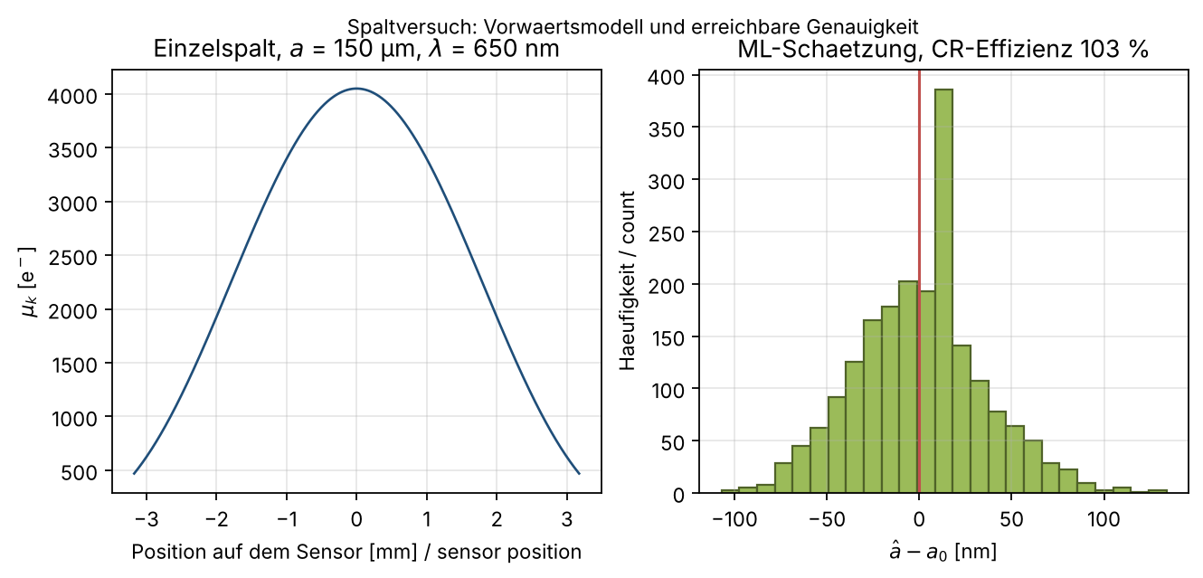
With this setup the slit width is estimable to about 36 nm, i.e. of its value. The decisive point for the experimental programme: accuracy is limited by photon statistics and model fidelity, not by pixel size.
For empirical testing of the separability criterion, the dependence on exposure and read noise serves:
| Exposure (scale factor) | at | at | at | at |
|---|---|---|---|---|
| 0.1 | ||||
| 1.0 | ||||
| 10 |
At high exposure is essentially proportional to exposure and independent of read noise — the product form holds. At low exposure the two parameters couple: the drop from to 30 is a factor of 8.4 there, but only 1.09 at tenfold exposure. Exactly this mixed dependence is measurable in the laboratory and is the test plan of Section 19.
| No. | Falsification case | Status v0.3 |
|---|---|---|
| 1 | Structure information at without near field, nonlinearity, priors, repeated measurement or a super-resolution mechanism | unchanged |
| 2 | Bearing reconstruction from a signal with without an additional channel | numerically demonstrated in 14.3 |
| 3 | New field frequencies in a demonstrably linear and time-invariant medium without nonlinear detection | LTV media excepted (Section 10) |
| 4 | Stable interference with genuinely absent coherence | unchanged |
| 5 | Reconstruction of lost analogue information from pure quantisation without additional information | unchanged |
| 6 | Energy or information balance that cannot be closed by reflection, transmission, absorption, scattering, frequency conversion or internal degrees of freedom | unchanged |
| 7 | Product form (9) holds in a system in which criterion (10) is demonstrably violated | testable per 14.7 and Section 19 |
| 8 | New: a stage efficiency stays constant across variation of upstream parameters although the noise model shows multi-stage injection | would refute Theorem 2 |
The framework stands in a tradition that begins in Vienna and leads via operationalism to modern model-based measurement theory. This placement is not decoration: it decides what the criterion may claim.
| Position | Core thesis | Standard criticism | What carries over |
|---|---|---|---|
| Mach (Analysis of Sensations 1886; economy of thought) | Physical concepts are economical summaries of elements; atoms are dispensable | Planck 1908/09; later confirmation of atomism by Perrin and Einstein | Economy of thought as minimal parametrisation — but no restriction to the observable, since may be theoretical |
| Boltzmann (picture theory, Populäre Schriften 1905) | Theories are pictures or models; several pictures may represent the same phenomena | — | Non-identifiability is precisely this model pluralism in statistical form. Boltzmann is the closest ancestor of the framework |
| Bridgman (The Logic of Modern Physics 1927) | A concept is synonymous with the corresponding set of operations | Every new measurement method creates a new concept; theoretical terms remain unexplained | The framework avoids the trap: is defined model-theoretically, the channel is only the test instance. The core statement is an exclusion criterion, not a definition of meaning |
| Vienna Circle: Carnap (Testability and Meaning 1936/37), Neurath, Schlick | Verifiability or confirmability criterion of meaning | Hempel 1950: too strict for universal statements, too liberal under disjunction | What carries: Carnap’s shift from verifiability to gradual confirmability — the counterpart to as a graded measure. What does not: a criterion of meaning for sentences |
| Schrödinger (1935) | Entanglement; the expectation catalogue of a subsystem is incomplete | — | Information resides only in the total state: Section 13 |
| Tal, Measurement in Science (SEP); model-based measurement theory | Measurement is process plus model; indication and measurement outcome must be separated | — | The framework is a model-based theory: = indication, = outcome, = model |
| Representational theory of measurement (Krantz, Luce, Suppes & Tversky 1971) | Measurement as homomorphism of empirical into numerical relations; uniqueness theorems | presupposes observable relations | Uniqueness theorems correspond to the equivalence classes of observational equivalence |
| GUM (JCGM 100:2008), VIM | Uncertainty propagation with sensitivity coefficients | linearisation | is a normalised sensitivity coefficient; corresponds to Type A uncertainty at the Cramér–Rao bound |
| Underdetermination (Duhem, Quine 1951); gauge freedom | Data do not determine theories uniquely; gauge directions are physically redundant | — | Gauge directions are exact null directions of the Fisher matrix; the identifiable structure is the quotient |
Position of the framework. It is a model-based, information-metric measurement theory. From Mach it takes economy, from Boltzmann model pluralism, from Carnap gradation. It avoids operationalism because it does not define meaning via operations but only excludes what no channel can distinguish. The classical objection to Mach — atoms were not directly observable and exist nonetheless — does not apply: atoms were identifiable through suitable channels, such as Brownian motion. Non-identifiability is channel-relative, not absolute. That sentence is the philosophical point of the framework and at the same time its safeguard against any positivist overreach.
| Framework | Object | Stochastic | Graded | Physical chain decomposition | Relation |
|---|---|---|---|---|---|
| Hadamard, Tikhonov, Bertero & Boccacci | well-posedness, regularisation | partly | via singular values | no | non-identifiability corresponds to the kernel of the forward operator |
| Identifiability (Koopmans; Rothenberg 1971) | observational equivalence | yes | locally via the Fisher matrix | no | supplies the core statement; no novelty here |
| Estimation theory (Kay 1993; Van Trees 1968) | Cramér–Rao, Fisher information | yes | yes | no | supplies |
| Kalman observability | rank of the observability matrix | no | binary | no | in the linear-Gaussian case the Fisher information of the initial state is the -weighted observability Gramian; full rank regular |
| Hermann & Krener (1977) | local weak observability, rank condition on Lie derivatives | no | binary | no | differential version; null directions are non-identifiable directions |
| Empirical Gramians, measures of unobservability (Krener & Ide 2009) | graded observability | partly | yes | no | closest graded competitor |
| Structural identifiability (Bellman & Åström 1970) | parameters from ideal data | no | binary | no | limiting case |
| Practical identifiability, profile likelihood (Raue et al. 2009) | finite, noisy data | yes | yes | no | methodologically closest |
| Cascaded DQE theory | signal and noise power per stage | yes | yes | yes | closest chain decomposition; denies the general product form |
Clean demarcation. Kalman and Hermann–Krener observability answer whether states are distinguishable from noise-free output trajectories of a dynamical system. The present framework asks how much information about each physical stage of a static or quasi-static measurement chain transmits under noise, and whether that transmission factorises stagewise. In the linear-Gaussian case the rank condition and the regularity of the Fisher matrix coincide; this equivalence is cited here as known and not presented as a result.
New relative to all of these are three points: the assignment of stages to physical sub-theories, the criterion for admissibility of the product form, and the treatment of the quantum stage with the distinction between POVM-bound and attainable information.
| Example | Lesson for measurability |
|---|---|
| mirror vs. matte wall | reflected energy is not directed information |
| clear vs. frosted glass | transparency is not structure transfer |
| microphone array | direction arises from time or phase differences, not from a local level |
| radar (civil: navigation, weather) | range, Doppler and bearing are different information channels |
| sonar (civil: bathymetry, fisheries) | multipath can supply information or create ambiguity |
| eddy-current testing | a defect is reconstructed via altered electromagnetic reaction, not seen |
| digital camera | a pixel value is the outcome of optics, sensor, gain, quantisation and processing; saturation destroys information |
| double slit | which-path information and interference capability must be described via measurement operators and coherence |
| parametric amplifier | new frequencies without nonlinearity; time variance is a channel of its own |
| cooled vs. uncooled camera | the same sensor moves between shot- and read-limited regimes — and thus between separable and non-separable |
The protocol is designed to be feasible in a workshop with 3D printing, a laser diode and a camera sensor, without laboratory equipment. It tests two things: the structure-transfer factor and the separability criterion.
| Component | Specification | Rationale |
|---|---|---|
| Light source | laser diode 635–650 nm, Class 2 ( mW) | fully sufficient with ND filters; Class 2 keeps the EN 60825-1 effort low |
| Slits | commercial slit set or two razor blades on a micrometer stage, 50–300 µm | FDM and resin printing give no defined edges below 100 µm |
| Distance | m, measured to mm | Fraunhofer condition , here 0.035 |
| Sensor | monochrome CMOS with RAW output, known pixel pitch | a Bayer matrix otherwise halves effective sampling |
| Tube and baffles | 3D printed, matte black, several stray-light baffles | stray light creates offset and lowers modulation |
| Neutral filters | ND series | exposure series without changing the geometry |
| Series | Variation | Purpose |
|---|---|---|
| R1 | slit width in 6–8 steps from 50 to 300 µm | over the range |
| R2 | exposure time over 3 decades at fixed | signal level |
| R3 | gain or read noise in 3–4 steps | |
| R4 | 30 repetitions per operating point with realignment | reproducibility and empirical variance |
The framework is supported if the mixed derivative differs significantly from zero in the crossover and not in the asymptotes. Theorem 2 would be refuted if stage efficiencies stayed constant across all operating points although the photon-transfer curve shows multi-stage noise injection.
| Regulation | Content |
|---|---|
| EN 60825-1:2014 + A11:2021 (IEC 60825-1:2014 Ed. 3.0 + AMD1/AMD2:2017) | classification and accessible emission limits; Class 2 in the visible up to 1 mW. An IEC 4th edition is in preparation and not yet published |
| IEC TR 60825-14:2022 (Ed. 2.0) | user guidance, hazard assessment |
| ISO 12233:2024 | resolution and spatial frequency response; supersedes the 2023 edition and carries a changed title |
| Directive 2006/25/EC, in Austria VOPST | workplace exposure limits |
| EN 208 | alignment eyewear for the visible range |
Anyone who alters or removes the optics of a classified laser module must reclassify and counts as a manufacturer under the standard. Exact limits are to be taken from the standard’s tables, not from secondary sources.
The utility of the framework lies in systematically separating signal, energy, information, direction, material response and decision. A bright image is not automatically information-rich. A null signal is not automatically absence. A digital reconstruction is not automatically physically unique.
Relative to version 0.2 the contribution shifts a second time. There, was derived but the validity of the product form was open. Here it is decided for the main channel classes, and the result is less comfortable than the product form suggests: factorisability is not a property of the system but of the operating point. The same camera is separable in bright light and not at dusk. That is not a weakness of the presentation but a statement about measurement chains, and it is measurable.
The mathematical core remains the measurement distribution . is a diagnostic tool for engineering use, not the theoretical core.
First, this is not a new fundamental theory. Second, the core statement is not new but adopted. Third, outside the Gaussian anchor case is an approximation. Fourth, the classification in Section 5.6 is not exhaustive; it covers the channel classes examined. Fifth, distinguishability in principle does not guarantee practical reconstructability. Sixth, information here means physical state distinguishability, not meaning. Seventh, all ten minimal models are simulations with known forward models; the experiment of Section 19 is planned, not performed. Eighth, the literature search was limited: “not found in the literature” does not mean “does not exist”. Ninth, not every reference has been verified at the work itself; Appendix I flags the open entries individually.
Measurability is distinguishable state dependence within a real physical measurement chain. The starting point — excludes unique reconstruction — is the observational equivalence of identifiability theory and is adopted here, not claimed. The own contribution is the stage decomposition of a physical measurement chain and the criterion stating when it may be collapsed multiplicatively.
The shortest version: measurability is distinguishable state dependence — and the product form holds exactly as far as its factors do not secretly contain one another. Whether they do is decided by the operating point, not by the instrument.
| Symbol | Meaning |
|---|---|
| , , | initial state, parameter to be estimated, measurement result |
| , , , , | chain operators and decision stage |
| signal-to-noise ratio | |
| , | wave-vector transfer, structure size |
| structure-transfer factor | |
| normalised state–signal coupling (elasticity); enters as | |
| material and propagation factor | |
| coherence factor (was in v0.1) | |
| bearing-information factor | |
| direction cosine (was in v0.1) | |
| signed direction balance (was in v0.1) | |
| , | effective SNR ; signed version |
| , | Fisher information, quantum Fisher information |
| stage efficiency | |
| , | reflection coefficient, standing-wave ratio |
| excess noise factor. Convention: carried here throughout as the variance factor ; Robbins & Hadwen (2003) define the amplitude quantity |
| Formula | Valid for | Caution with |
|---|---|---|
| harmonic waves with defined phase velocity | strong dispersion | |
| plane or locally plane waves | strongly localised fields | |
| scattering, reflection, diffraction with definable wave vectors | strongly diffuse fields | |
| coarse structure resolution | near field, super-resolution, strong priors | |
| passive linear systems without gain | active media, frequency conversion, time-varying media | |
| pure post-processing | priors, training data, sensor fusion | |
| standard form of outcome probabilities | not a complete interpretation of the measurement problem | |
| scalar Gaussian channel | any coupling of signal and noise | |
| only where separability (10) holds; class A exact, B asymptotic | class C: multi-stage noise, aperture, nonlinearity, crossover regime | |
| stage-intrinsic | class A | once noise at the chain end dominates (14.6) |
| two counter-propagating components along one axis | multimode fields | |
| qubit, pure dephasing, phase estimation | additional relaxation, multi-qubit systems |
cd werkzeuge
python3 FORSCH-PROV0420_minimalmodelle_v0.2_2026-08-26_numerik.py   # M1-M6, seed 20260826
python3 FORSCH-PROV0420_minimalmodelle_v0.3_2026-10-05_numerik.py   # M7-M10, seed 20261005
Dependencies: Python 3, numpy, matplotlib.
The scripts write ergebnisse.json and
ergebnisse_v0.3.json and all figures to
werk/abb/. Every number in Section 14 comes from these
files.
Every entry carrying an identifier (DOI, ISBN, bibcode) was confirmed for this version with the publisher, the registration agency’s record, or the full text. Entries without an identifier are standard textbooks whose edition is still to be fixed; they are listed as open in Appendix I.
| Version | Change |
|---|---|
| v0.1 → v0.2 | dimensioned and derived; separability criterion introduced; falsification case 3 tightened to LTI; notation decoupled (, , , ); identified with VSWR; null space extended to the singular-value continuum; identifiability named; six numerical models; DOIs added; spelling Bertero & Boccacci corrected; bilingual DE+EN |
| v0.8 → v0.9 | nothing in the work itself; the bundle made ready for publication:
VEROEFFENTLICHUNG.md as the sequence in one place, landing
page extended with legal matters and the network of brands, citation
template in the author register raised from Version 0.3 to the current
version |
| v0.7 → v0.8 | new Appendix G.6: self-protection and the disclosure line per REGEL-PROV0002; for every component it is stated whether it is open and why; checkability outranks protection recorded as the precedence; the choice for the browser tool made and justified |
| v0.6 → v0.7 | new Appendix G.5: active and passive versions per the cross-track rule REGEL-PROV0001; the borderline case of computation scripts settled in favour of checkability; the difference between free verification and the licensed tool stated |
| v0.5 → v0.6 | commercial arrangement converted to a platform-centred one: Appendix G rewritten (syntagma-science as the destination, the open channel as the feeder), licence levels L0–L3 and six product classes per LIZ-PROV0001 added, Appendix H reordered to platform → deposit → journals, Zenodo bundle prepared separately; tools run exclusively on the platform |
| v0.4 → v0.5 | source check carried out and folded in (verified entries 23 → 50, open 25 → 12): ISO 12233 corrected to the 2024 edition with its changed title; IEC TR 60825-14 dated to 2022 (Ed. 2.0) and the status of IEC 60825-1 Ed. 4 noted; the conference paper WSA 2010 replaces the arXiv preprint as the primary source for one-bit quantisation; journal name corrected for Kalman (1963); six missing DOIs added; issue numbers added for ten entries; Appendix D converted into one continuous alphabetical list; Appendix I structured into verified / still open / what the check changed; open entries reduced from 25 to 13 |
| v0.3 → v0.4 | gap claim tied to the strands searched; class C extended by three cases; noise coefficient and Stam inequality demarcated; Section 7.1 (Rayleigh and Sparrow as thresholds); convention for the excess noise factor fixed; quantum bounds under noise and QFI monotonicity added; Appendix H (publication path) and Appendix I (source checklist) new; twelve references added |
| v0.2 → v0.3 | core statement identified as observational equivalence; Theorem 1 with proof; Theorem 2 (stage formulation); classification A/B/C; demarcation from Cox–Reid and DQE; four new minimal models M7–M10; experimental protocol; Vienna lineage; demarcation from observability theory; Appendices F and G new |
The following list belongs to the integrity of the contribution. It states what could not be found after reviewing the strands data-processing inequality, cascaded systems and detective quantum efficiency, quantisation, detector noise, parameter orthogonality, information geometry, observability theory and structural identifiability. The search comprised roughly two dozen targeted queries; it was not exhaustive and does not replace a systematic review. “Not found” does not mean “does not exist”. Every statement in this appendix is qualified accordingly in the text.
| Sought | Status |
|---|---|
| General criterion for cascaded measurement chains | not found; the DQE literature explicitly denies the general product form |
| “Separable” or “multiplicative Fisher information” as a named concept | not found |
| Information geometry of the model family over the instrument-parameter space (fibre bundle) | not found |
| Existence theorem for a mixing reparametrisation making separable | not found |
| Teaching experiment with a radiometrically calibrated raw sensor and an estimate of Cramér–Rao efficiency | not found |
| Philosophical work explicitly treating gauge orbits as the null space of the Fisher metric | not found |
This work is run platform-centred. The platform syntagma-science is where everything converges; the open research channel feeds it rather than being the destination.
| Track | Content | Licence | Location | Role |
|---|---|---|---|---|
| syntagma-science (platform) | the MESSWERK tool in two editions, documentation, training, measurement-chain audit, design work | licensed, levels L0–L3 | syntagma-science/, syntagma-science.com |
Destination. Every tool runs here, this is where purchases and installations happen |
| FORSCHUNG / Syntagma Forschung | this preprint, figures, computation scripts, raw results | CC BY 4.0, open | werk/, zenodo-upload/,
forschung.tschueller.com |
Feeder. Substantiates the method openly and leads to the platform |
Tools run exclusively on the platform. No tool is deposited on Zenodo, not even a preview or demonstration build — what is deposited there is the preprint with figures, scripts and raw results. Anyone who wants to compute rather than read comes to the platform.
Following the licence and platform scheme LIZ-PROV0001.
| Level | What it covers | For this work |
|---|---|---|
| L0 — open | freely readable, CC BY 4.0, no registration | preprint in all four formats, both languages, nine figures, both computation scripts, both raw-result files |
| L1 — read | platform registration, bundle access, version tracking | curated reading view of the work with cross-references into the tool modules |
| L2 — apply | tool use, updates, support | MESSWERK universal, six computation modules, single seat or embedding |
| L3 — install | multi-seat, own branding, training, audit | MESSWERK white-label, measurement-chain audit, design against a required accuracy |
| Class | Filled in this project by | Level |
|---|---|---|
| Preprint | the present work | L0 |
| Monograph | not filled — an expanded book is conceivable but not begun | — |
| Tool Basic | MESSWERK universal, six browser modules | L2 |
| Tool Pro | MESSWERK with own branding, multi-seat, data import from photon-transfer calibration | L3 |
| Course | half-day training “measurability instead of signal strength” | L2/L3 |
| Institutional licence | technical college, university of applied sciences, test laboratory: tool plus training plus audit | L3 |
The open preprint is a publication and reach channel, not an end in itself: it substantiates the method openly so that the platform rests on something checkable. Every deposit of the preprint carries the reference to syntagma-science. Both tracks are maintained; neither replaces the other. The identifiers FORSCH-PROV0420 and SYN-PROV0002 are provisional and are to be checked against the register before publication.
The assignment follows the cross-track rule
REGEL-PROV0001 (version 1.0 of 6 Oct 2026, text in
regelwerk/). It governs all projects, not only this
one.
Only the passive version goes on the deposit. The active version runs exclusively on the platform.
| Active → platform only | Passive → deposit permitted | |
|---|---|---|
| Mark | has an operating surface and computes, decides or produces in response to input | is read, viewed, or run once for verification |
| In this project | MESSWERK in both editions, six browser computation modules | this work in four formats per language, nine figures, both computation scripts, both raw-result files |
The test, in this order: does it have an operating surface that computes on input? If yes, active. If no: is it read, viewed, or run once for verification? If yes, passive.
The computation scripts of Appendix C are passive and go on the deposit. A fixed-seed script that regenerates the numbers of Section 14 is reproduction material, not an application. Without it this work could not be checked, and checkability is the reason for depositing at all. Anyone who wants to verify the numbers here does not need MESSWERK; the scripts suffice. MESSWERK removes the setup work and computes on someone else’s measurement chain rather than on the examples of this work — that is the difference the licence rests on.
Never on the deposit: preview, demonstration and reduced builds of the tool, the tool’s source including its surface, offering and pricing material, and internal files. Either the full tool on the platform or none at all.
The line between what lies open and what stays with the author
follows the cross-track rule REGEL-PROV0002 (version
1.0 of 6 Oct 2026, text in regelwerk/). It is named here
because this work sits beside a paid offering, and the question would
otherwise go unstated.
The line runs at the subject, not the format: the method this work claims and substantiates is public. Without evidence it would be advertising, not research. The product sold alongside it is protected.
| Subject | Status | Reason |
|---|---|---|
| Theorems 1 and 2 with proofs, classification A/B/C | open | this is the claim; publishing it without proof would be worthless |
| Computation scripts M1–M10 with fixed seeds | open | they regenerate every number of Section 14; without them the work cannot be checked |
| Experimental protocol, Section 19 | open | it describes how to refute the theory, not how to build the product. It names component classes, not suppliers, and refers calibration to the public EMVA 1288 standard rather than to in-house correction tables |
| Own calibration data, correction tables, suppliers, part numbers | not present | under REGEL-PROV0002 these stay internal in any case; they are not needed here and appear nowhere |
| Prices, cost prices, costing | not present | price levels belong in the licence scheme LIZ-PROV0001, not in a preprint |
Checkability outranks protection. Where a detail is needed to keep the claim refutable, it is published, even where a third party benefits. A framework that cannot be refuted supports no offering.
A browser tool, deliberately open. MESSWERK runs as
a single HTML file in the browser and therefore ships its computing core
to everyone who opens the page. “In the browser” and “core source
internal” exclude each other; REGEL-PROV0002 accordingly requires a
deliberate choice per tool. For MESSWERK the choice has been made and is
recorded in syntagma-science/ANGEBOT.md: the
universal edition stays open on the platform page. The licence
then carries not the computing core but maintenance and version
tracking, own branding and multi-seat operation, training, the
measurement-chain audit and design against a required accuracy. This is
not a fallback but the decision to weigh the funnel higher than the
protection of a few hundred lines of computation code that are derivable
from this work anyway.
Platform first, deposit second, journals last.
| Step | What | Why in this order |
|---|---|---|
| 1 | Set up syntagma-science: work page, MESSWERK in the universal edition, documentation, licence levels | the platform is the destination; every later reference has to point somewhere |
| 2 | Deposit the Zenodo bundle
(zenodo-upload/) with a DOI, CC BY 4.0, and the reference
to the platform in both the description and the work |
secures priority and citability; carries readers onward |
| 3 | Submit the individual articles, each referring to the deposit | review takes time; priority is already secured by then |
The working bundle and the publication bundle are not the same thing.
The folder zenodo-upload/ holds exactly what belongs on the
deposit and nothing else: preprint in four formats per language,
figures, computation scripts, raw results, licence, metadata record,
read-me. It does not hold tool builds, offering and pricing material,
internal handovers or checklists. The bundle’s metadata name the
platform as the related identifier.
| Venue | Fit | Requirements |
|---|---|---|
| syntagma-science.com | the destination | own platform, no external requirements; licence levels per Appendix G.2 |
| Zenodo with ORCID | immediately possible, subordinate | no endorsement, DOI on request; suitable for the bilingual monograph; the description points to the platform |
arXiv physics.data-an, cross-list eess.SP,
quant-ph, physics.hist-ph |
high, but with a hurdle | Endorsement required. Since 21 Jan 2026 automatic endorsement requires both an institutional e-mail address and a prior publication in the same endorsement domain. In physics each subject class is its own domain. Without both, a personal endorsement by an established arXiv author of the same domain is needed; operations staff cannot endorse |
| Entropy | high for the mathematical core | open access; an article processing charge applies on acceptance (CHF 2600 per the publisher) |
| Measurement Science and Technology | medium to high once the experiment exists | requires experimental validation |
| Metrologia | medium | only with a clear link to GUM and VIM |
| European Journal of Physics, American Journal of Physics | high for the experimental part | teaching-lab focus; Section 19 is already cut for this |
| Synthese, Studies in History and Philosophy of Science | for the philosophical part | requires philosophical originality beyond the placement |
A single work covering mathematics, experiment and philosophy of science fits no single journal. Splitting it into three submissions is more workable, with the bilingual monograph as the common, openly accessible deposit:
| Article | Content | Target |
|---|---|---|
| 1 | Theorem 1, Theorem 2, classification A/B/C, models M1, M4, M7, M8 | Entropy or a correspondence in an information-theory journal |
| 2 | experimental protocol, models M3 and M10, photon-transfer calibration | European Journal of Physics |
| 3 | Sections 16 and 17, expanded | Synthese or Studies in History and Philosophy of Science |
Status verified means the entry was confirmed for this version against the publisher’s record, the standards register, the full text, or the registration agency’s entry. open means the entry is still not individually substantiated and is to be confirmed before a journal version. The check was carried out on 6 Oct 2026.
| Source | Identifier | Evidence |
|---|---|---|
| Rothenberg (1971) | DOI 10.2307/1913267 | publisher |
| Cox & Reid (1987) | DOI 10.1111/j.2517-6161.1987.tb01422.x | publisher |
| Zamir (1998) | DOI 10.1109/18.669301 | publisher |
| Braunstein & Caves (1994) | DOI 10.1103/PhysRevLett.72.3439 | publisher |
| Helstrom (1969) | DOI 10.1007/BF01007479 | publisher |
| Kullback & Leibler (1951) | DOI 10.1214/aoms/1177729694 | publisher |
| Morgenthaler (1958) | DOI 10.1109/TMTT.1958.1124533 | publisher |
| Friis (1944) | DOI 10.1109/JRPROC.1944.232049 | publisher |
| Rabbani, Shaw & Van Metter (1987) | DOI 10.1364/JOSAA.4.000895 | publisher |
| Cunningham, Westmore & Fenster (1994) | DOI 10.1118/1.597401 | publisher |
| Cunningham & Shaw (1999) | DOI 10.1364/JOSAA.16.000621 | publisher — formed from the publisher’s pattern in v0.4, now confirmed |
| Robbins & Hadwen (2003) | DOI 10.1109/TED.2003.813462 | publisher |
| Hynecek & Nishiwaki (2003) | DOI 10.1109/TED.2002.806962 | publisher |
| Chao, Ward & Ober (2012) | DOI 10.1007/s11045-011-0150-7 | publisher |
| Mortensen et al. (2010) | DOI 10.1038/nmeth.1447 | publisher |
| Escher et al. (2011) | DOI 10.1038/nphys1958 | publisher |
| Raue et al. (2009) | DOI 10.1093/bioinformatics/btp358 | publisher |
| Hermann & Krener (1977) | DOI 10.1109/TAC.1977.1101601 | publisher |
| Krener & Ide (2009) | DOI 10.1109/CDC.2009.5400067 | publisher — listed as missing in v0.4 |
| Quine (1951) | DOI 10.2307/2181906 | publisher |
| Zurek (2003) | DOI 10.1103/RevModPhys.75.715 | publisher |
| Schrödinger (1935), Parts I and II | DOI 10.1007/BF01491891, 10.1007/BF01491914 | publisher |
| Gan & Law (2009) | DOI 10.1088/0143-0807/30/6/006 | publisher |
| Aspden, Padgett & Spalding (2016) | DOI 10.1119/1.4955173 | publisher |
| Bertero & Boccacci (1998) | ISBN 978-0-7503-0435-1 | publisher (spelling Boccacci) |
| Chernoff (1952) | DOI 10.1214/aoms/1177729330 | publisher |
| Amari (2001) | DOI 10.1109/18.930911 | publisher |
| Amari (2016) | DOI 10.1007/978-4-431-55978-8 | publisher |
| Paris (2009) | DOI 10.1142/S0219749909004839; issue 7(Suppl. 1) added | publisher |
| Hughston, Jozsa & Wootters (1993) | DOI 10.1016/0375-9601(93)90880-9 | publisher |
| Kalman (1963) | DOI 10.1137/0301010; journal name corrected to J. Soc. Ind. Appl. Math., Series A: Control | publisher |
| Bellman & Åström (1970) | DOI 10.1016/0025-5564(70)90132-X; issue 7(3–4) added | publisher |
| Worrall (1989) | DOI 10.1111/j.1746-8361.1989.tb00933.x | publisher |
| Earman & Norton (1987) | DOI 10.1093/bjps/38.4.515 | publisher |
| Carnap (1936/37) | DOI 10.1086/286432 and 10.1086/286443 | publisher |
| Mezghani, Antreich & Nossek (2010) | DOI 10.1109/WSA.2010.5456454; WSA 2010, Bremen, 143–150 | publisher — the conference paper is now the primary source, arXiv:1010.5532 the preprint |
| Galiffi et al. (2022) | DOI 10.1117/1.AP.4.1.014002 | publisher — no DOI in v0.4 |
| Hansen (1998) | DOI 10.1137/1.9780898719697 | publisher — no DOI in v0.4 |
| Janesick (2007) | DOI 10.1117/3.725073 | publisher — ISBN only and unverified in v0.4 |
| Stadler (2015) | DOI 10.1007/978-3-319-16561-5 | publisher — ISBN only and unverified in v0.4 |
| Landauer (1991) | DOI 10.1063/1.881299; issue 44(5) | publisher |
| Shannon (1948) | DOI 10.1002/j.1538-7305.1948.tb01338.x and 10.1002/j.1538-7305.1948.tb00917.x; issues 27(3) and 27(4) | publisher |
| Berreman (1972) | DOI 10.1364/JOSA.62.000502; issue 62(4) | publisher |
| Hempel (1950) | Revue Internationale de Philosophie 4(11), 41–63 | full-text evidence via the collective review in the Journal of Symbolic Logic |
| Trimmer (1980) | JSTOR 986572 | publisher — no DOI has been assigned |
| Sparrow (1916) | bibcode 1916ApJ….44…76S | full text in the ADS archive |
| Rayleigh (1879) | DOI 10.1080/14786447908639684 | publisher |
| ISO 12233:2024 | standard, 5th edition | ISO register — replaces ISO 12233:2023; the title also changed: “Digital cameras — Resolution and spatial frequency responses” instead of “Photography — Electronic still picture imaging — …” |
| IEC TR 60825-14:2022 (Ed. 2.0) | standard | IEC register |
| IEC 60825-1:2014 Ed. 3.0 + AMD1/AMD2:2017; EN 60825-1:2014 + A11:2021 | standard | IEC register — a 4th edition stands at stage 30.60 (close of voting 2 Oct 2026) and is not published |
| Source | Identifier | Status |
|---|---|---|
| Abbe (1873) | Arch. mikrosk. Anat. 9(1), 413–468 | open — issue and page range from the secondary literature; no DOI on record |
| Schrödinger (1935), Part III | — | open — no DOI is on record for the third part |
| Goodman, Introduction to Fourier Optics | edition and ISBN | open — the edition is to be fixed before the journal version |
| Kay (1993) | ISBN | open |
| Green & Swets (1966) | ISBN | open |
| Krantz et al. (1971) | ISBN of the reprint | open |
| Tikhonov & Arsenin (1977) | ISBN | open |
| Born & Wolf; Boyd; Cover & Thomas; Jackson; Mandel & Wolf; Nielsen & Chuang; Pozar; Van Trees; Woodward | edition and ISBN | open — standard textbooks with no edition-bound passage cited in this work |
| Boltzmann (1905), Mach (1886), Bridgman (1927) | first editions | open — edition not checked against a copy |
| JCGM 100:2008, JCGM 200:2012 | BIPM | open — edition status not checked against the document |
| EMVA 1288 Release 4.0 | standard | open — valid module designation not checked against the standard text |
| Tal, Measurement in Science (SEP) | version date | open — the SEP is revised continuously; an access date is to be added |
| Item | v0.4 | v0.5 |
|---|---|---|
| Standard for the MTF measurement | ISO 12233:2023 | ISO 12233:2024, 5th edition, with a changed title |
| Laser safety guidance | IEC TR 60825-14 without a year | IEC TR 60825-14:2022, Ed. 2.0 |
| One-bit quantisation | arXiv preprint as the source | conference paper WSA 2010 with a DOI as the primary source |
| Kalman (1963) | SIAM Journal on Control | J. Soc. Ind. Appl. Math., Series A: Control — the present journal name is the later one |
| open entries | 25 | 12, almost exclusively edition and ISBN questions |
| verified entries | 23 | 50 |